SPF AlgorithmSPF 演算法

A metric is an indication of the overhead that is required to send packets across a certain interface. OSPF uses cost as a metric. A smaller cost indicates a better path than a higher cost. By default on Cisco devices, the cost of an interface is inversely proportional to the bandwidth of this interface, so a higher bandwidth indicates a lower cost. For example, there is more overhead, a higher cost, and more time delays that are involved in crossing a 10-Mbps Ethernet line than in crossing a 100-Mbps Ethernet line.

度量值（metric）表示透過某介面傳送封包所需的額外負擔。OSPF 使用成本（cost）作為度量值。成本越小代表路徑越好。在 Cisco 裝置上，介面的成本預設與該介面的頻寬成反比，因此頻寬越高，成本越低。舉例來說，通過 10 Mbps 乙太網路線路所涉及的額外負擔、較高的成本，以及較長的時間延遲，都比通過 100 Mbps 乙太網路線路來得多。

On Cisco devices, the formula used to calculate OSPF cost is cost = reference bandwidth / interface bandwidth (in bits per second).

在 Cisco 裝置上，計算 OSPF 成本的公式是：成本 = 參考頻寬 / 介面頻寬（以 bps 為單位）。

The default reference bandwidth is 10⁸, which is 100,000,000, or the equivalent of the bandwidth of Fast Ethernet. Therefore, the default cost of a 10-Mbps Ethernet link will be 10⁸ / 10⁷ = 10, and the cost of a 100-Mbps link will be 10⁸ / 10⁸= 1. The problem arises with links that are faster than 100 Mbps. Because the OSPF cost has to be an integer, all links that are faster than Fast Ethernet will have an OSPF cost of 1.

預設參考頻寬為 10⁸，也就是 100,000,000，相當於快速乙太網路的頻寬。因此，10 Mbps 乙太網路鏈路的預設成本為 10⁸ / 10⁷ = 10，而 100 Mbps 鏈路的成本為 10⁸ / 10⁸= 1。問題出在比 100 Mbps 更快的鏈路上。因為 OSPF 成本必須是整數，所有比快速乙太網路更快的鏈路，其 OSPF 成本都會是 1。

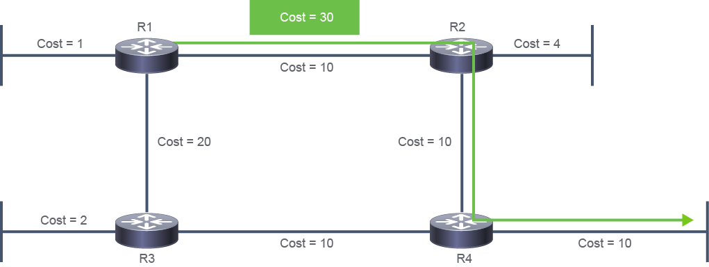
The cost to reach a distant network from a router is the cumulative cost of all links on the path from the router to the network. In the example, the cost from R1 to the destination network via R3 is 40 (20 + 10 + 10), and the cost via R2 is 30 (10 + 10 + 10). The path via R2 is better because it has a lower cost.

從某路由器到達遠端網路的成本，是從該路由器到目的網路路徑上所有鏈路成本的累加值。在此範例中，R1 經由 R3 到達目的網路的成本為 40（20 + 10 + 10），經由 R2 的成本為 30（10 + 10 + 10）。經由 R2 的路徑較佳，因為它的成本較低。

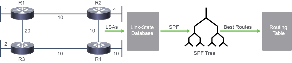
The figure represents the R1 view of the network, where R1 is the root and calculates the pathways by assuming this view.

此圖代表 R1 對網路的視角，其中 R1 是根節點，並根據此視角來計算路徑。

Each router has its own view of the topology even though all the routers build the shortest path trees by using the same LSDB.

即使所有路由器都使用相同的 LSDB 來建立最短路徑樹，每台路由器仍有各自的拓樸視角。

Each router places itself as the root of a tree and then runs the SPF algorithm. The path calculation is based on the cumulative cost that is required to reach that destination. LSAs are flooded throughout the area by using a reliable algorithm, which ensures that all the routers in an area have the same LSDB (topological database). Because of the flooding process, R1 has learned the link-state information for each router in its area. Each router uses the information in its topological database to calculate a shortest path tree, with itself as the root. The router then uses this tree to determine the best routes, which are offered to the routing table to route network traffic.

每台路由器都會將自己置於樹的根節點，然後執行 SPF 演算法。路徑計算是根據到達該目的地所需的累加成本。LSA 會透過可靠的演算法在區域內泛洪，以確保區域內所有路由器都擁有相同的 LSDB（拓樸資料庫）。由於泛洪程序的緣故，R1 已學習到其區域內每台路由器的鏈路狀態資訊。每台路由器都使用其拓樸資料庫中的資訊，以自己為根節點計算最短路徑樹。路由器接著使用此樹來決定最佳路由，並提供給路由表以路由網路流量。

For R1, the best path to each LAN and its cost are shown in the table. Note that in terms of number of hops (routers) to reach the destination, the shortest path might not necessarily be the best one, because the selection of the best route is based on the lowest total cost value from the available paths. Each router has its own view of the topology, even though the routers build shortest-path trees by using the same LSDB.

表中列出 R1 到各 LAN 的最佳路徑及其成本。請注意，就到達目的地所需的躍點（路由器）數量而言，最短路徑不一定就是最佳路徑，因為最佳路由的選擇是根據可用路徑中最低的總成本值。即使所有路由器都使用相同的 LSDB 建立最短路徑樹，每台路由器仍有各自的拓樸視角。